Section 21 SVD and Image Compression
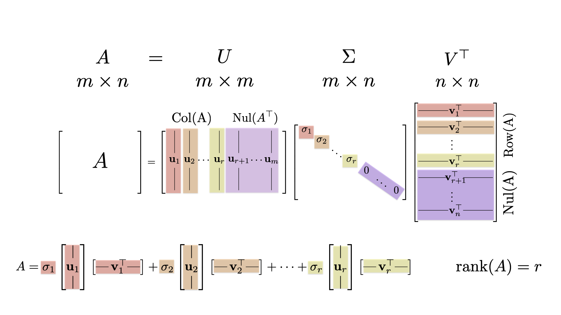
Here we will illustrate one application of the singular value decomposition SVD of a matrix \(A\). To learn more about this, and other cool applications, take MATH 365 Computational Linear Algebra.
21.1 Example
Here is a \(4 \times 5\) matrix \(A\).
(A = cbind(c(1,-1,1,0),c(-2,3,0,2),c(1,-1,1,0),c(0,1,4,0),c(1,-1,5,-4)))## [,1] [,2] [,3] [,4] [,5]
## [1,] 1 -2 1 0 1
## [2,] -1 3 -1 1 -1
## [3,] 1 0 1 4 5
## [4,] 0 2 0 0 -4We will call svd(A,nv=ncol(A)) to compute the singular value decomposition. (The nv=ncol(A) forces svd to give us all of the columns. For technical reasons, the default output does not).
svd(A,nv=ncol(A))## $d
## [1] 7.657063e+00 4.528454e+00 1.965323e+00 1.981025e-16
##
## $u
## [,1] [,2] [,3] [,4]
## [1,] -0.2248593 0.3962930 -0.4593417 -0.7624929
## [2,] 0.2098332 -0.7003225 0.3056557 -0.6099943
## [3,] -0.8000554 -0.5005874 -0.2933731 0.1524986
## [4,] 0.5150919 -0.3192373 -0.7807125 0.1524986
##
## $v
## [,1] [,2] [,3] [,4] [,5]
## [1,] -0.1612561 0.13161844 -0.5385224 0.1709288 -0.7984047
## [2,] 0.2754845 -0.77996334 0.1395320 -0.4039829 -0.3648207
## [3,] -0.1612561 0.13161844 -0.5385224 -0.7769031 0.2511736
## [4,] -0.3905399 -0.59682006 -0.4415746 0.4039829 0.3648207
## [5,] -0.8482805 -0.02856877 0.4533541 -0.2019914 -0.1824103The singular value decomposition (SVD) is the matrix factorization \[ A = U \Sigma V^T \qquad \hbox{or} \qquad U^T A V = \Sigma, \] where \(\Sigma\) is the \(4 \times 5\) matrix with the singular values down the column. We can confirm this with the following computation that gives the matrix \(\Sigma\).
U = svd(A,nv=ncol(A))$u
V = svd(A,nv=ncol(A))$v
zapsmall(t(U) %*% A %*% V)
## [,1] [,2] [,3] [,4] [,5]
## [1,] 7.657063 0.000000 0.000000 0 0
## [2,] 0.000000 4.528454 0.000000 0 0
## [3,] 0.000000 0.000000 1.965323 0 0
## [4,] 0.000000 0.000000 0.000000 0 0The spectral decomposition is \[ A = \sigma_1 \mathsf{u}_1 \mathsf{v}_1^{\top} + \sigma_2 \mathsf{u}_2 \mathsf{v}_2^{\top} + \sigma_3 \mathsf{u}_3 \mathsf{v}_3^{\top} + \sigma_4 \mathsf{u}_4 \mathsf{v}_4^{\top}. \]
For example, we can get the first matrix in this deccomposition as
##            [,1]       [,2]       [,3]       [,4]      [,5]
## [1,]  0.2776445 -0.4743187  0.2776445  0.6724166  1.460537
## [2,] -0.2590912  0.4426227 -0.2590912 -0.6274829 -1.362938
## [3,]  0.9878667 -1.6876386  0.9878667  2.3924763  5.196629
## [4,] -0.6360087  1.0865360 -0.6360087 -1.5403248 -3.345696
21.2 Image Compression
We need the jpeg package.
We will use the cameraman image, which is a famous photo from image and signal processing.
where = "https://www.macalester.edu/~dshuman1/data/cameraman_small.jpg"
img = readJPEG(readBin(where,"raw",1e6))
dim(img)
## [1] 256 256The matrix img is a 256 x 256 matrix with each entry representing the grayscale value of a single pixel. So to store the image, we need to store 65,536 floating point numbers. We can plot it with the following function:
imPlot = function(img,...) {
  plot(1:2, type='n',xlab=" ",ylab= " ",...)
  rasterImage(img, 1.0, 1.0, 2.0, 2.0)
}
imPlot(img,main="Cameraman Image")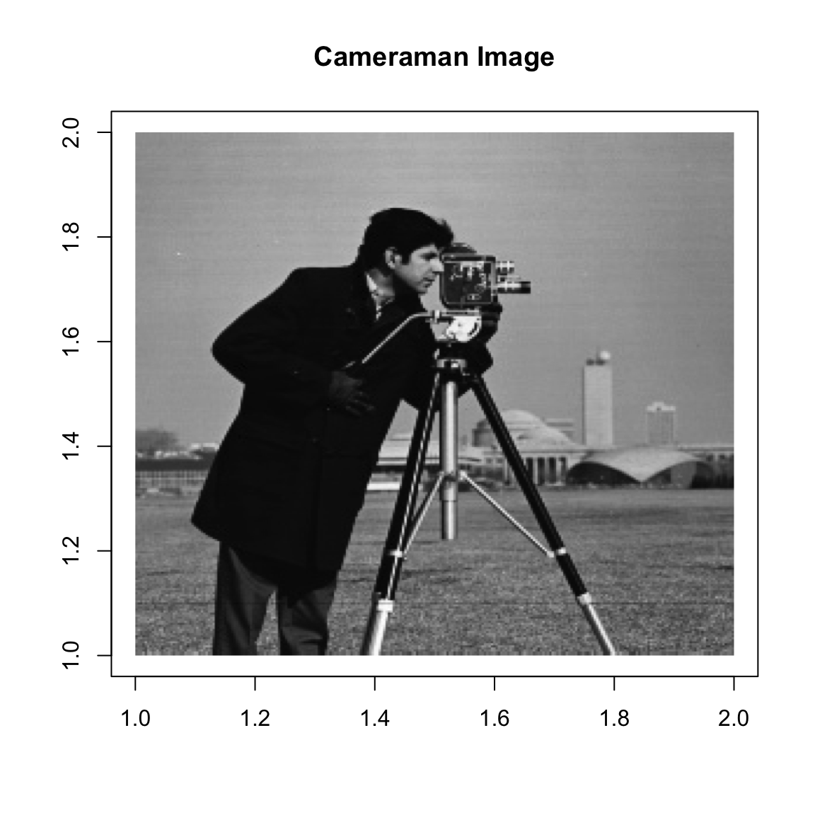
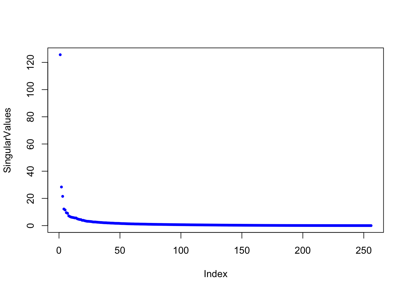
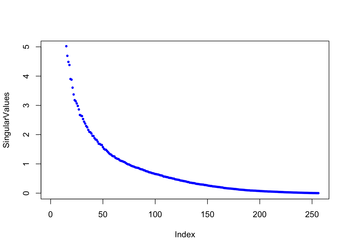
Here are the singular values of the image
The following code is used to choose only the first \(k\) singular values in the spectral decomposition.
SVDApprox = function(A,k = floor(1/2*min(nrow(A),ncol(A)))) {
  foo = svd(A)
  sings = foo$d
  U = foo$u
  V = foo$v
  if(k==1)
    D=matrix(sings[1],nrow=1,ncol=1)
  else
    D=diag(sings[1:k])
  M=U[,1:k]%*%D%*%t(V[,1:k])
  return(M)
}
approxImg=function(img,k){
  approxIm = SVDApprox(img,k)
  approxIm[approxIm<0] = 0
  approxIm[approxIm>1] = 1
  plot(1:2, type='n')
  rasterImage(approxIm, 1.0, 1.0, 2.0, 2.0)
}
And here we show the singular value approximation with increasing numbers of singular values:
approxImg(img,1)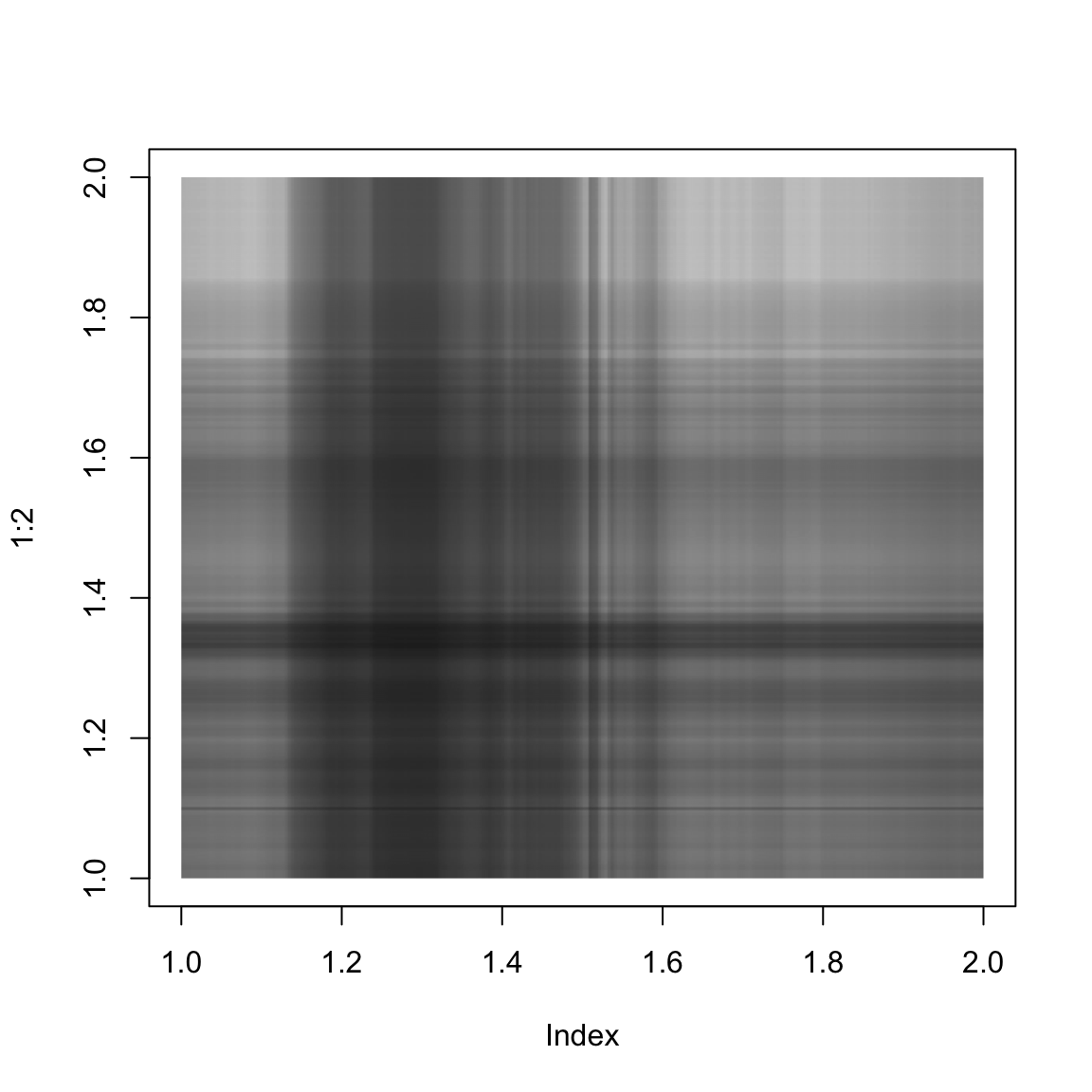
approxImg(img,2)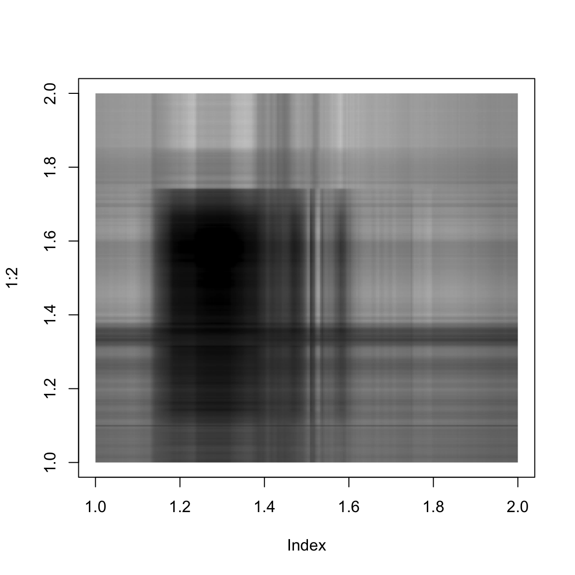
approxImg(img,3)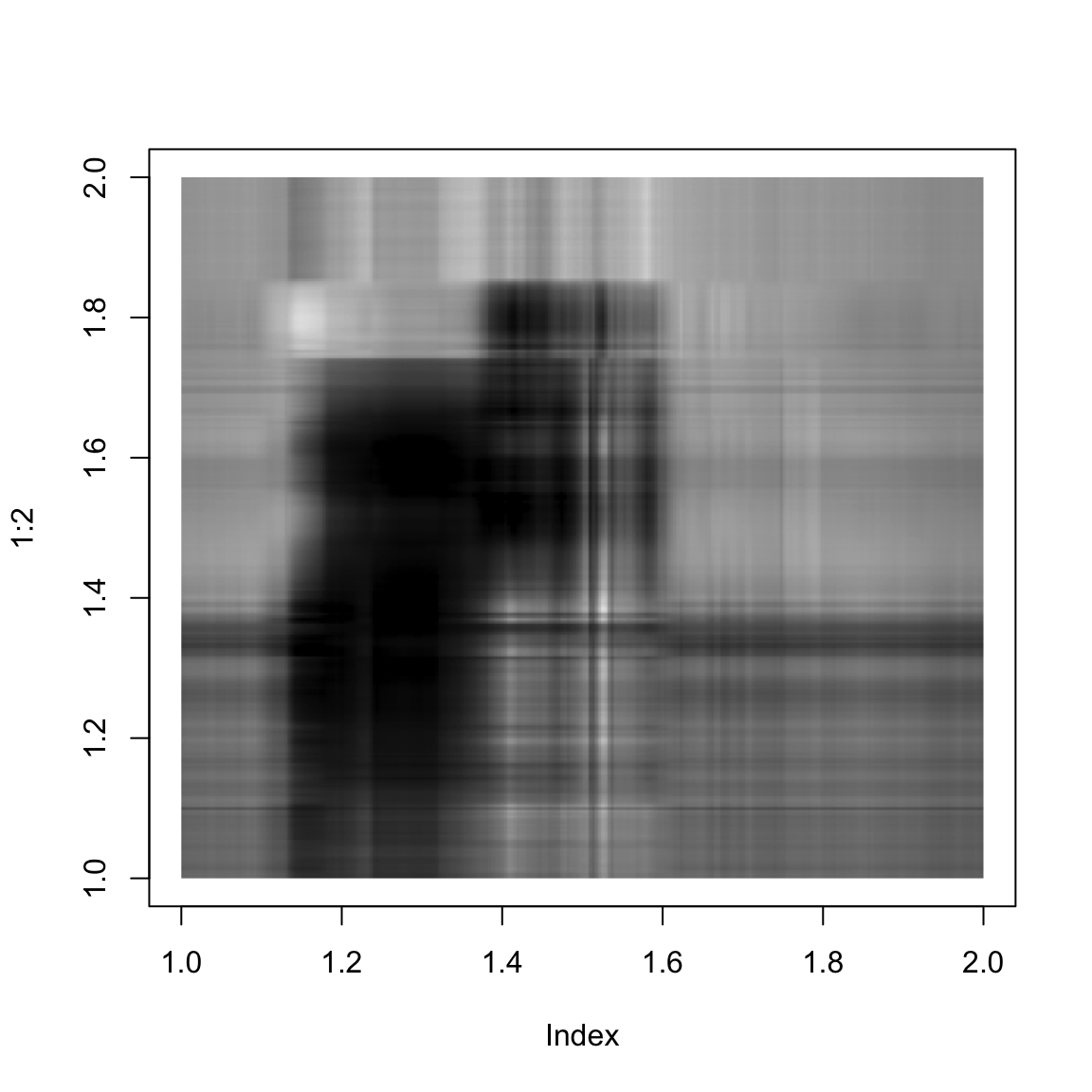
approxImg(img,4)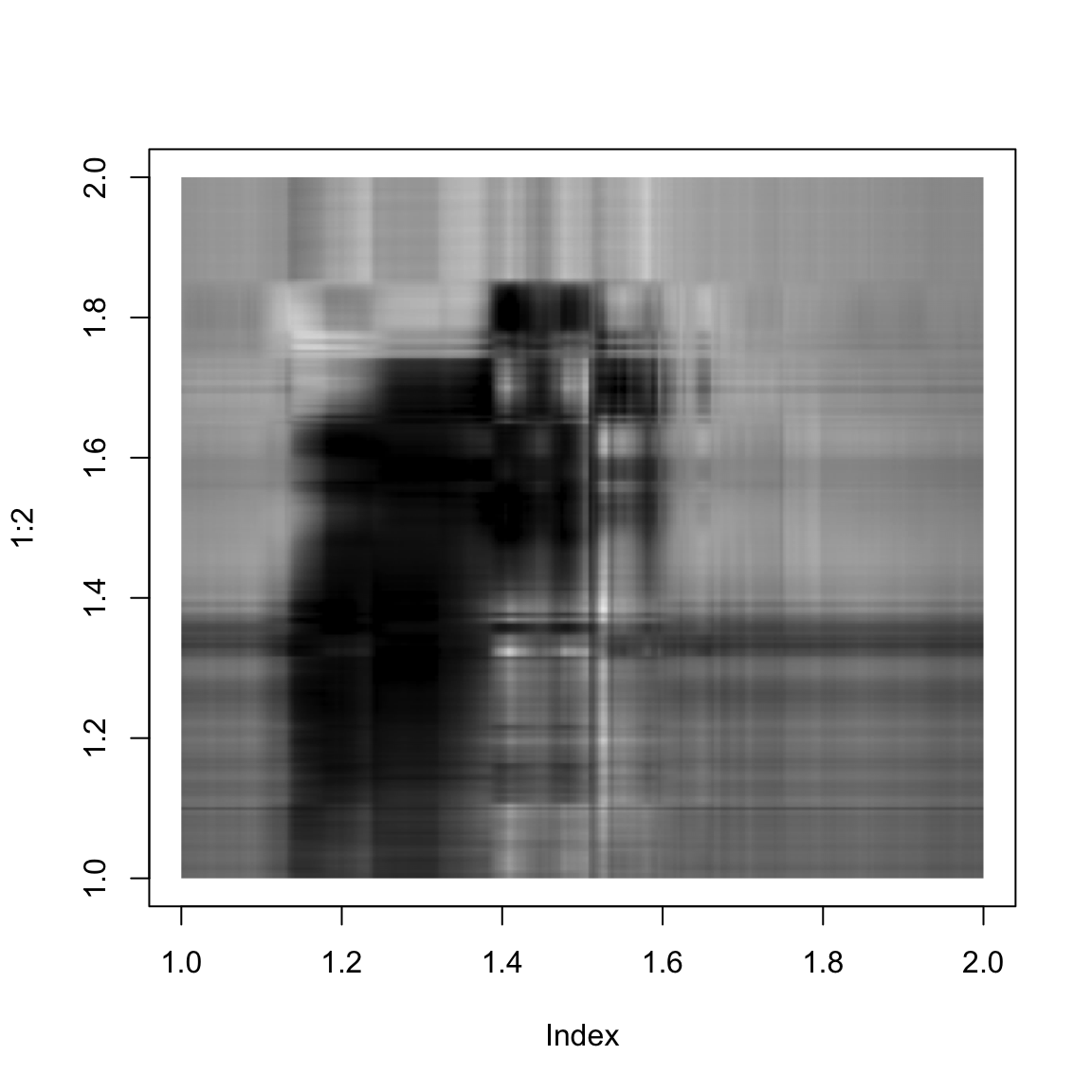
approxImg(img,5)
approxImg(img,10)
approxImg(img,25)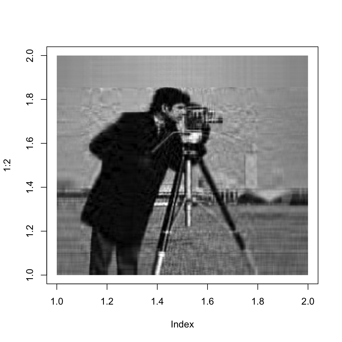
approxImg(img,50)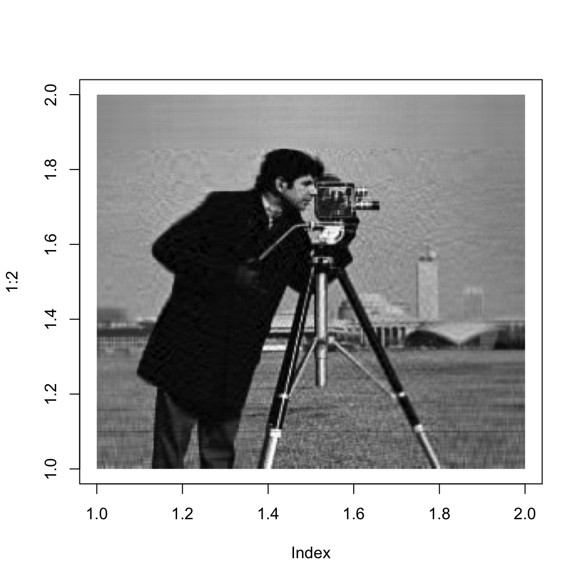
approxImg(img,100)