Section 7 Problem Set 7

Last one! You can drop your lowest problem set, so if you are happy with 6 problem set scores you can drop this one. However, I recommend you work on and think about these problems, since these ideas will be on the final quiz.
Due: Wednesday July 07 by 11:59am CST (last day of class).
Upload your solutions to Moodle in a PDF.
Please feel free to use RStudio for all calculations, including row reduction, matrix multiplication, eigenvector calculation and inverse matrices.
You can download the Rmd source file for this problem set.

This problem set covers Network Centralities and Sections 6.1, 6.2, 6.3, 6.5 on Orthogonal Projections.

7.1 Orthogonal Complements

(Work on in class on Tuesday June 29)

Here are two subspaces of $\mathbb{R}^5$ that we have seen before. (See PS4.2 and PS5.2) \[ \begin{align} \mathsf{Z} & = \left\{ \begin{bmatrix} x_1 \\ x_2 \\ x_3 \\ x_4 \\ x_5 \end{bmatrix} \ \bigg\vert \ x_1 + x_2 + x_3 + x_4 + x_5 = 0, x_4 = 2 x_2 \right\}. \\ \mathsf{F} & = \left\{ \begin{bmatrix} x_1 \\ x_2 \\ x_3 \\ x_4 \\ x_5 \end{bmatrix} \ \bigg\vert \ x_3 = x_1 + x_2, x_4 = x_2 + x_3, x_5 = x_3 + x_4 \right\}. \end{align} \] Find the orthogonal complement of each subspace in $\mathbb{R}^5$. For each example, compute $\dim(W) + \dim(W^\perp)$.

7.2 Cosine Similarity

(Work on in class on Tuesday June 29)

In high dimensional space $\mathbb{R}^n$ a common measure of similarity between two vectors is cosine similarity: the cosine of the angle $\theta$ between the vectors. We calculate this value as shown below. This formula was derived in the video for 5.1. \[ \cos(\theta) = \frac{ \mathsf{u} \cdot \mathsf{v}} {\| \mathsf{u}\| \, \|\mathsf{v}\|} = \frac{ \mathsf{u} \cdot \mathsf{v}} {\sqrt{\mathsf{u} \cdot \mathsf{u}} \sqrt{\mathsf{v} \cdot \mathsf{v}}}. \] This measure has the following nice properties:

$-1 \le \cos(\theta) \le 1$,
$\cos(\theta)$ is close to 1 if $\mathsf{u}$ and $\mathsf{v}$ are closely aligned,
$\cos(\theta)$ is close to 0 if $\mathsf{u}$ and $\mathsf{v}$ are are orthogonal,
$\cos(\theta)$ is close to $-1$ if $\mathsf{u}$ and $\mathsf{v}$ are polar opposites.
$\cos(\theta)$ is positive if $\theta$ is acute (less than $90^o$).
$\cos(\theta)$ is negative if $\theta$ is obtuse (greater than $90^o$).

Write a function cosine_similarity that takes as input two vectors $\mathsf{u}$ and $\mathsf{v}$ and returns the value of $\cos(\theta)$ for the angle $\theta$ between $\mathsf{u}$ and $\mathsf{v}$. Below is a shell of the code that you need. Right now it always just returns 1.You need to fix that up. Demonstrate that your code works on some vectors in $\mathbb{R}^5$. Use vectors that are orthogonal, closely aligned, and close to polar opposites.

cosine_similarity <- function(u, v) {
  # your code goes here!
  # find the cosine of the angle between u and v
  cosine = 1
  return (cosine)
}

In the file US_Senate_s21.Rmd you will find vectors of the voting record of the Senate in the 109th US Congress (2007-2008). You will see how to take the dot product of the voting record of two different senators. The dot product is always an integer. Explain what it counts. It is the number of something or possibly the difference of two things.
Use your cosine_similary function to find the cosine similarity between every pair of the following senators:
- Hilary Clinton (D, NY), presidential candidate 2016
- John McCain (R, AZ), presidential candidate 2008
- Barack Obama (D, IL), president 2008-2016
- Susan Collins (R, ME), moderate Republican

Does the cosine similarity pick up on the fact that Senator Collins is a “moderate Republican”?

The senate majority leader of the 109th Congress was Bill Frist (R, TN), and the senate minority leader was Harry Reid (D, NV).
- Create a function classify_senator(senator) that returns “R” or “D” depending on the cosine similarity of senator to frist and to reid. You will have to write an “if … else statement” (here is the syntax).
- There is a chunk of code in the R file I’ve given you that gets you started.
- Then run the my_classification code that we have given. I dentify any senators that have been misclassified using this method, meaning that their votes are more similar to the leader of the opposing party.
- Jim Jeffords (I, VT) was a Republican who became and Independent in 2001 and then caucused with the Democrats. How does your classifier handle Jeffords?

7.3 Orthogonal Diagonalization

(Work on in class on Wednesday June 30)

Recall that a square $n \times n$ matrix is symmetric when $A^{\top} = A$. It is an amazing property that the eigenvectors of a symmetric matrix form an orthogonal basis of $\mathbb{R}^n$. In this problem, you will confirm that this holds for the following symmetric matrix, \[ A = \begin{bmatrix} 0 & 8 & 10 & -4 \\ 8 & 4 & 28 & 6 \\ 10 & 28 & 3 & -4 \\ -4 & 6 & -4 & -7 \end{bmatrix}. \]

A = cbind(c(0,8,10,-4),c(8,4,28,6),c(10,28,3,-4),c(-4,6,-4,-7))

Find the eigenvalues and eigenvectors of $A$.
Let $P$ be the matrix of the eigenvectors output by R: P = eigen(A)$vectors. Confirm that these eigenvectors are an orthonormal set using a single matrix calculation.
Let $\mathsf{v} = \begin{bmatrix} 2 & -4 & -9 & -2 \end{bmatrix}^{\top}$. Find the coordinates of $\mathsf{v}$ in the eigenbasis in 3 different ways:
1. Use the transpose of $P$. Recall that, in R, the transpose of a matrix is t(A).
2. Augment and row reduce.
3. Use the dot product formula. Note that the command v1 = P[,1] will extract the first eigenvector from the matrix P.
Diagonalize $A$ using $P$. To demonstrate this compute both $A= P D P^{-1}$ and $D =P^{-1} A P$. Congratulations: you have orthogonally diagonalized the symmetric matrix $A$!

Turn in: Your R code and the output for each part.

7.4 Fibonacci Orthogonality

(Work on in class on Thursday July 1)

In problem 4.2, you saw that the vector space of Fibonacci vectors $\mathsf{F} \subseteq \mathbb{R}^5$ is a 2-dimensional subspace of $\mathbb{R}^5$.

Below is an orthogonal basis of $\mathsf{F}$. Check that the basis vectors $\{\mathsf{f}_1, \mathsf{f}_2\}$ are in $\mathsf{F}$ and are orthogonal. \[ \mathsf{F} = \mathsf{span} \left\{ \mathsf{f}_1 = \begin{bmatrix} 1 \\ 0 \\ 1 \\ 1 \\ 2 \end{bmatrix}, \mathsf{f}_2 = \begin{bmatrix} -9 \\ 7 \\ -2 \\ 5 \\ 3\end{bmatrix} \right\}, \hskip.5in \mathsf{v} = \begin{bmatrix} 1 \\ 2 \\ 3 \\ 5 \\ 7\end{bmatrix}.\hskip.5in \]
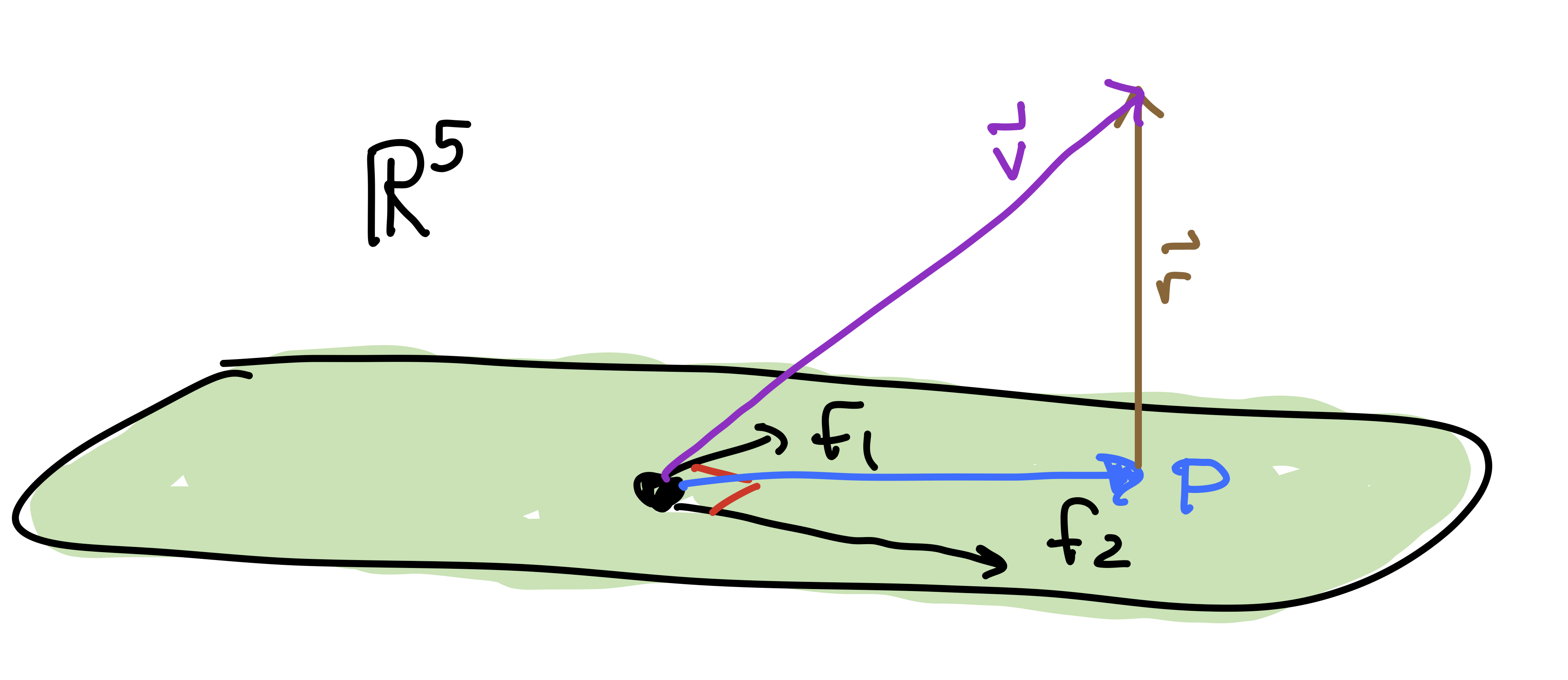
The vector $\mathsf{v}$ above is not in $\mathsf{F}$ (check that!). Its projection $\mathsf{p}$ onto $\mathsf{F}$ is given by the formula below. Compute $\mathsf{p}$. This is closest approximation of $\mathsf{f}$ with a Fibonacci vector. \[ \mathsf{p} = \frac{ (\mathsf{v} \cdot \mathsf{f}_1)}{ ( \mathsf{f}_1 \cdot \mathsf{f}_1)} \mathsf{f}_1 + \frac{ (\mathsf{v} \cdot \mathsf{f}_2)}{ ( \mathsf{f}_2 \cdot \mathsf{f}_2)} \mathsf{f}_2. \] This formula requires that the basis be orthogonal.
The residual vector is the vector $\mathsf{r} = \mathsf{v} - \mathsf{p}$. Compute $\mathsf{r}$.
Show that $\mathsf{r}$ is orthogonal to $\mathsf{f}_1$ and $\mathsf{f}_2$.
Compute $||\mathsf{r}||$. This is the distance from $\mathsf{v}$ to $\mathsf{F}$ (i.e., how far $\mathsf{v}$ is from being Fibonacci?).

7.5 Least Squares Solution to $\mathsf{A} x = \mathsf{b}$

(Work on in class on Tuesday July 6)

Find the least-squares solution to the following inconsistent matrix equation $\mathsf{A} x = \mathsf{b}$. \[ \left[ \begin{array}{ccc} 1 & 1 & 2 \\ 1 & 0 & 2 \\ -1 & 1 & 1 \\ 1 & 0 & 1 \\ 1 & 1 & 1 \\ \end{array} \right] \begin{bmatrix} x_1 \\ x_2 \\ x_3 \end{bmatrix} = \begin{bmatrix} 7 \\ 11 \\ -3 \\ 10 \\ 7 \end{bmatrix}. \hskip5in \] Here are the steps you should follow:

Show that this system of equations is inconsistent.
Make the normal equations: $\mathsf{A}^T \mathsf{A} x = \mathsf{A}^T \mathsf{b}$.
Solve the normal equations for $\hat{x}$ (by hand or software).
Get the projection $\hat{\mathsf{b}}$ of $\mathsf{b}$ onto $\mathrm{Col}(\mathsf{A})$ by $\hat{\mathsf{b}} = \mathsf{A} \hat{x}$.
Get the residual $\mathsf{r} = \mathsf{b} - \hat{\mathsf{b}}$ and compute its length.

7.6 Least-Squares Polynomials

(Work on in class on Tuesday July 6)

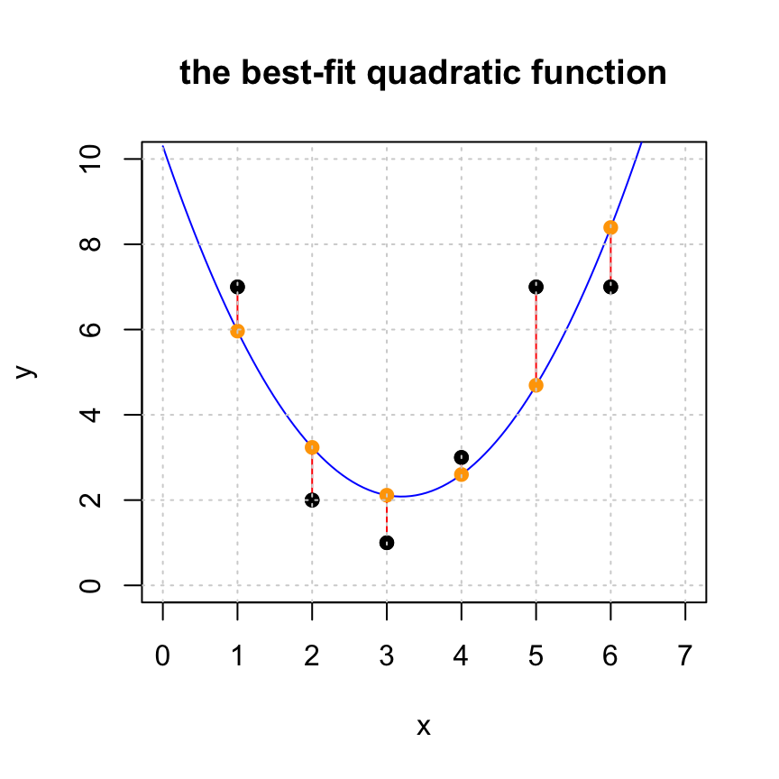
Here is a quadratic least-squares polynomial fit to some data. Make a cubic, quartic, and quintic fit to this same data. Turn in a plot of each. Compute the length of the residual in each case. Which do you think is the best model of the data?

x = c(1,2,3,4,5,6)
y = c(7,2,1,3,7,7)
(A = cbind(x^0,x,x^2))

##        x   
## [1,] 1 1  1
## [2,] 1 2  4
## [3,] 1 3  9
## [4,] 1 4 16
## [5,] 1 5 25
## [6,] 1 6 36

xhat = solve(t(A)%*%A,t(A)%*%y)
yhat = A %*% xhat
r = y - yhat
t(r) %*% r

##          [,1]
## [1,] 11.26429

#plot the original set of points
plot(x,y,pch=19,xlim=c(0,7),ylim=c(0,10), main='the best-fit quadratic function')
# generate points for the fitted line and plot it
tt = seq(0,7,len=100)  
lines(tt,xhat[1]+xhat[2]*tt+xhat[3]*tt^2,col='blue')
# add the residuals to the plot
for (i in 1:length(x)) {lines(c(x[i],x[i]),c(y[i],yhat[i]), col='red')}
#add yhat to the plot
points(x,yhat,pch=19,col='orange')
#put the original points back on the plot last so we can see them 
points(x,y,pch=19,col="black")
grid()

7.7 Fuel Efficiency

(Work on in class on Wednesday July 7)

Below is a classic data set of fuel efficiency in 38 different automobiles.

##                            lbs  HP Cyl  MPG
## BuickEstateWagon       3967.60 155   8 16.9
## FordCountrySquireWagon 3689.14 142   8 15.5
## ChevyMalibuWagon       3280.55 125   8 19.2
## ChryslerLeBaronWagon   3585.40 150   8 18.5
## Chevette               1961.05  68   4 30.0
## ToyotaCorona           2329.60  95   4 27.5
## Datsun510              2093.00  97   4 27.2
## DodgeOmni              2029.30  75   4 30.9
## Audi5000               2575.30 103   5 20.3
## Volvo240GL             2857.40 125   6 17.0
## Saab99GLE              2543.45 115   4 21.6
## Peugeot694SL           3103.10 133   6 16.2
## BuickCenturySpecial    3075.80 105   6 20.6
## MercuryZephyr          2793.70  85   6 20.8
## DodgeAspen             3294.20 110   6 18.6
## AMCConcordD/L          3103.10 120   6 18.1
## ChevyCapriceClassic    3494.40 130   8 17.0
## FordLTD                3389.75 129   8 17.6
## MercuryGrandMarquis    3599.05 138   8 16.5
## DodgeStRegis           3485.30 135   8 18.2
## FordMustang4           2352.35  88   4 26.5
## FordMustangGhia        2648.10 109   6 21.9
## MazdaGLC               1797.25  65   4 34.1
## DodgeColt              1742.65  80   4 35.1
## AMCSpirit              2429.70  80   4 27.4
## VWScirocco             1810.90  71   4 31.5
## HondaAccordLX          1942.85  68   4 29.5
## BuickSkylark           2429.70  90   4 28.4
## ChevyCitation          2361.45 115   6 28.8
## OldsOmega              2457.00 115   6 26.8
## PontiacPhoenix         2325.96  90   4 33.5
## PlymouthHorizon        2002.00  70   4 34.2
## Datsun210              1838.20  65   4 31.8
## FiatStrada             1938.30  69   4 37.3
## VWDasher               1992.90  78   4 30.5
## Datsun810              2561.65  97   6 22.0
## BMW320i                2366.00 110   4 21.5
## VWRabbit               1925.00  71   4 31.9

Fit a linear model of the form \[ mpg = a_0 + a_1 lbs + a_2 HP + a_3 Cyl. \] Find the coefficients $a_0,a_1,a_2,a_3$ and the length of the residual. If you have taken Stat 155, you can see that we are doing the exact same thing by comparing your results with

## 
## Call:
## lm(formula = MPG ~ lbs + HP + Cyl)
## 
## Residuals:
##     Min      1Q  Median      3Q     Max 
## -4.4669 -1.6011 -0.3246  1.0759  6.6231 
## 
## Coefficients:
##              Estimate Std. Error t value Pr(>|t|)    
## (Intercept) 49.644579   1.992433  24.917  < 2e-16 ***
## lbs         -0.008288   0.002316  -3.579  0.00106 ** 
## HP          -0.073961   0.043862  -1.686  0.10091    
## Cyl          0.791590   0.730326   1.084  0.28604    
## ---
## Signif. codes:  0 '***' 0.001 '**' 0.01 '*' 0.05 '.' 0.1 ' ' 1
## 
## Residual standard error: 2.791 on 34 degrees of freedom
## Multiple R-squared:  0.833,  Adjusted R-squared:  0.8183 
## F-statistic: 56.55 on 3 and 34 DF,  p-value: 2.656e-13

Add the cars weight in tons to your model and solve $mpg = a_0 + a_1 (lbs) + a_2 (HP) + a_3 (Cyl) + a_4 (tons).$ Compare the coefficients you get with those that you got in part a. Give a short explanation of what you see using some of the linear algebra language that we have learned in the course.
The residual vector $\mathsf{r}$ measures the quality of fit of our model. But how do we turn this into a meaningful quantity? One method is to look at the coefficient of determination, which is more commonly refered to as the “$R^2$ value.”

You can see the $R^2$ value of your fit in part (a) under the “Multiple R-squared” output in the linear model summary above.
If $\mathsf{y} = [ y_1, y_2, \ldots, y_n ]^{\top}$ is our target vector with least-squares solution $\hat{\mathsf{y}} = A \hat{\mathsf{x}}$ and residual vector is $\mathsf{r} = \mathsf{y} - \hat{\mathsf{y}}$. Let \[ a = \frac{1}{n} ( y_1 + y_2 + \cdots + y_n) \] be the average or mean of the entries of target vector $\mathsf{y}$ and let $\mathsf{y}^* = [a, a, \ldots, a]$. (We call this vector “y star”, so ystar would be a fine name in R.) The $R^2$ value is \[ R^2 = 1 - \frac{\| \mathsf{y} - \hat{\mathsf{y}} \|^2 }{\| \mathsf{y} - \mathsf{y}^* \|^2} = 1 - \frac{\| \mathsf{r} \|^2}{\| \mathsf{y} - \mathsf{y}^* \|^2}. \]
The $R^2$ value is a number in $[0,1]$. The squared-length $|| \mathsf{y} -\mathsf{y}^*||^2$ is the total variance: that is, how much the data varies from the mean, and $\frac{\| \mathsf{r} \|^2}{\| \mathsf{y} - \mathsf{y}^* \|^2}$ tells us the fraction of the total variance that is explained by our model. Thus, if $R^2$ is near 1, then our model does a good job at “explaining” the behavior of $\mathsf{y}$ via a linear combination of the columns of $A$.
To do: Find the $R^2$ value for our least squares solution to the cars data in part (a). Here are some helpful functions: + mean(vec) returns the mean (average) of the entries of the vector vec + rep(a, n) creates a constant vector of length $n$ where every entry is $a$. + Norm(vec) from the pracma package returns the magnitude (Euclidean length) of the vector vec. To learn more, you should take STAT 155: Introduction to Statistical Modeling.

7.8 Fourier Analysis

(Work on in class on Wednesday July 7)

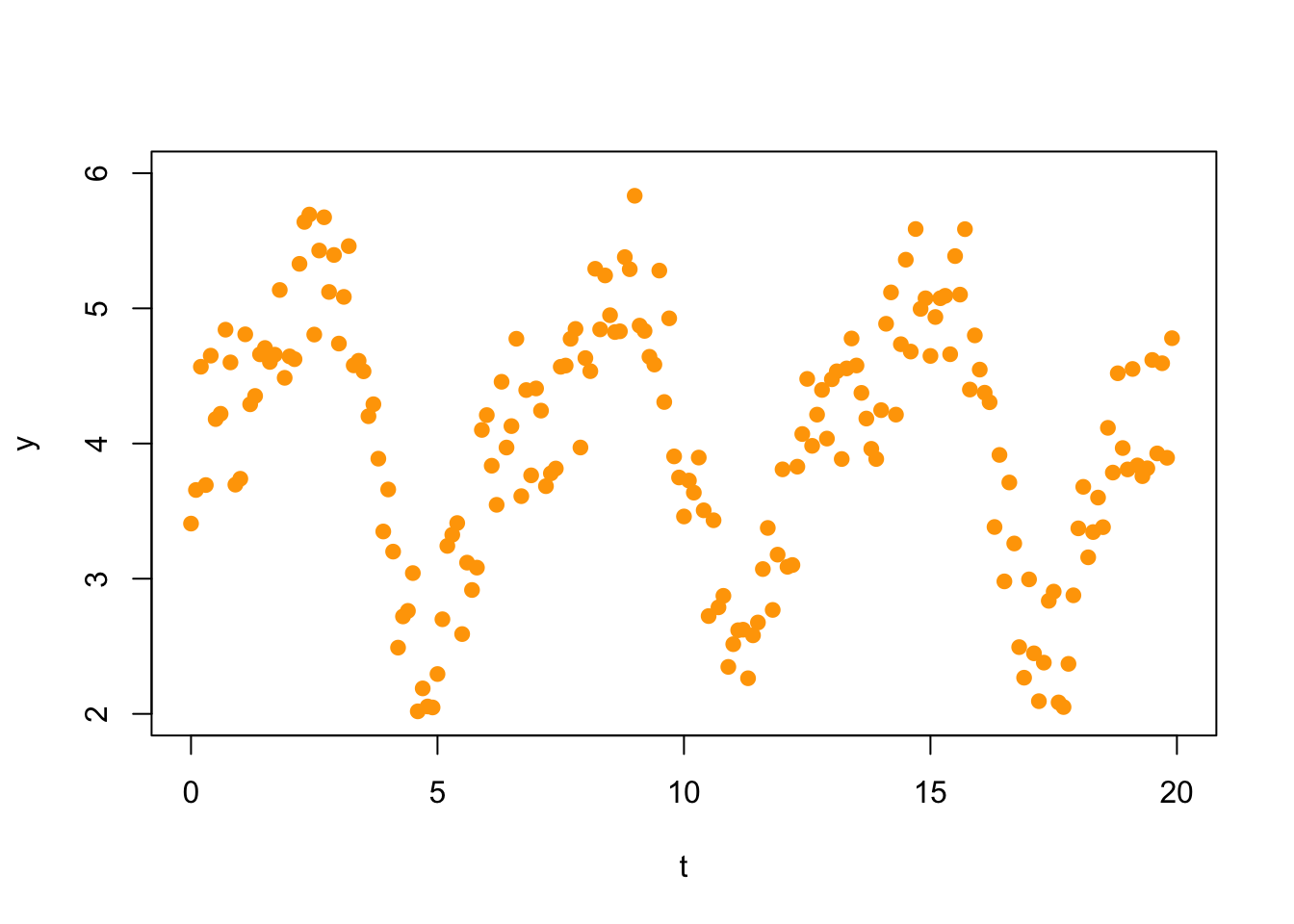
In Fourier analysis one uses trigonometric functions to model oscillatory behavior in data. These methods have important applications in the study of sound or video signals, financial data, medicine, and engineering (to mention just a few). For example, consider the following set of 200 data points.

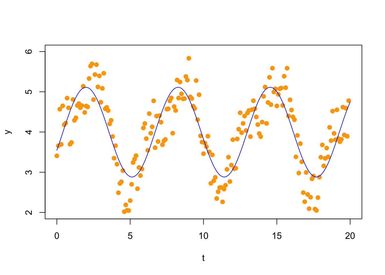
A first Fourier approximation would fit a model of the form \[ f_1(t) = c_0 + c_1 \sin(t) + c_2 \cos(t). \] Thus, we make the following matrix (we show here only the first 10 rows; there are 200 rows).

##       [,1]       [,2]      [,3]
##  [1,]    1 0.00000000 1.0000000
##  [2,]    1 0.09983342 0.9950042
##  [3,]    1 0.19866933 0.9800666
##  [4,]    1 0.29552021 0.9553365
##  [5,]    1 0.38941834 0.9210610
##  [6,]    1 0.47942554 0.8775826
##  [7,]    1 0.56464247 0.8253356
##  [8,]    1 0.64421769 0.7648422
##  [9,]    1 0.71735609 0.6967067
## [10,]    1 0.78332691 0.6216100

Now we solve the normal equations

##            [,1]
## [1,]  3.9971143
## [2,]  1.0207277
## [3,] -0.4486618

and plot the solution Your task:

Update this to add the second Fourier coefficient terms by fitting the following function to the data. Plot your result. \[ f_2(t) = c_0 + c_1 \sin(t) + c_2 \cos(t) + c_3 \sin(2t) + c_4 \cos(2t) \]
Compute the length of the residul vector for both the $f_1(t)$ and the $f_2(t)$ model. Which approximation looks better visually. That is, does the second approximation capture more of the shape of the data, or do you think that the first is a better model?

MATH 236: Linear Algebra