Section 8 Problem Set 8
Download the Rmd source file for this problem set.
Upload a completed, knitted .html version of this file on Moodle. If you have collaborated with others on this assignment (encouraged), please include their names here (no penalty).
8.1 Subspace Projection
Last week we learned how to project onto a subspace, but our method required that we have an orthogonal basis. Here we will see that our least-squares method allows us to project onto a subspace with any (not-necessarily-orthgoonal) basis. Consider the following subspace of \(\mathbb{R}^4\). We can turn it into a least-squares problem by making it the column space of a matrix \(A\). That is \(W = Col(A)\). \[ W = span\left\{ \begin{bmatrix} 1 \\ 2 \\ -1 \\ -2 \end{bmatrix}, \begin{bmatrix} 1 \\ 2 \\ 3 \\ 4 \end{bmatrix}, \begin{bmatrix} 1 \\ 0 \\ 1 \\ 0 \end{bmatrix} \right\}, \hskip.6in b = \begin{bmatrix} 9 \\ 5 \\ 5 \\ 8 \end{bmatrix}. \]
##      [,1] [,2] [,3]
## [1,]    1    1    1
## [2,]    2    2    0
## [3,]   -1    3    1
## [4,]   -2    4    0
Perform a matrix computation on A to show that the basis is not orthogonal.
Show that b is not in W.
Find the least-squares projection of b onto W. Find both \(\hat x\) and \(\hat b\).
Calculate the residual vector r, show that \(r \in W^\perp\), and find \(||r||\).
Consider the following derivation from the normal equations: \[ A^T A x = A^T b \qquad \Longrightarrow \qquad \hat x = (A^T A)^{-1} A^T b. \] The pseudoinverse is the matrix \[ A^+ = (A^T A)^{-1} A^T \] From what we see above it gives the least-squares solution to \(A x = b\). Compute the matrix \(A^+\), multiply it by \(b\), and show that you get \(\hat x\).
Continuing this story, \[ \hat b = A \hat x \qquad \Longrightarrow \qquad \hat b = A (A^T A)^{-1} A^T b. \] The projection matrix onto the subspace \(W\) is the matrix \[ P = A (A^T A)^{-1} A^T. \] Compute the matrix \(P\), apply it to \(b\), and see that you get the projected value \(\hat b\).
Compute \(P^2\) and compare it to \(P\). Explain why this happens.
Use \(P\) to project the vector
b2 = c(1,2,3,4)onto \(W\).Find the eigenvalues of \(P\). They are nice. Explain (briefly) where the eigenvectors of this matrix are in relation to \(W\).
8.2 Least-Squares Polynomials
Here is the problem that we discussed in class with a quadratic fit to it. Make a cubic, quartic, and quintic fit to this data. Turn in a plot of each. Comupute the length of the residual in each case. Which do you think is the best model of the data?
##        x
## [1,] 1 1  1
## [2,] 1 2  4
## [3,] 1 3  9
## [4,] 1 4 16
## [5,] 1 5 25
## [6,] 1 6 36## [,1]
## [1,] 11.26429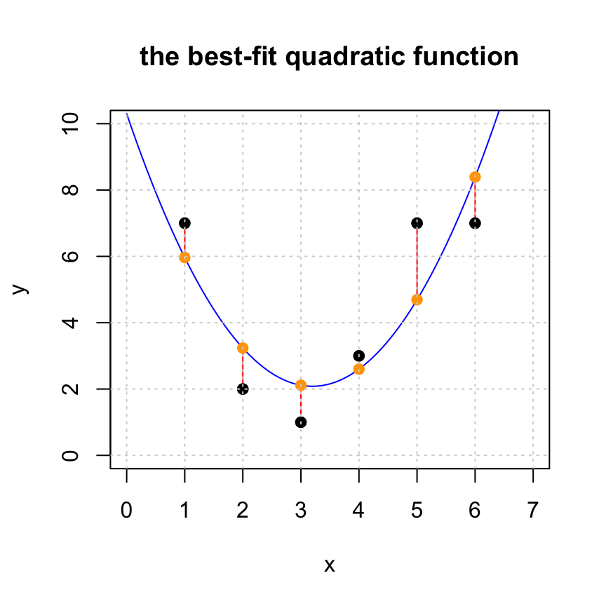
8.3 Fuel Efficiency
Below is a classic data set of fuel efficiency in 38 different automobiles.
##                            lbs  HP Cyl  MPG
## BuickEstateWagon       3967.60 155   8 16.9
## FordCountrySquireWagon 3689.14 142   8 15.5
## ChevyMalibuWagon       3280.55 125   8 19.2
## ChryslerLeBaronWagon   3585.40 150   8 18.5
## Chevette               1961.05  68   4 30.0
## ToyotaCorona           2329.60  95   4 27.5
## Datsun510              2093.00  97   4 27.2
## DodgeOmni              2029.30  75   4 30.9
## Audi5000               2575.30 103   5 20.3
## Volvo240GL             2857.40 125   6 17.0
## Saab99GLE              2543.45 115   4 21.6
## Peugeot694SL           3103.10 133   6 16.2
## BuickCenturySpecial    3075.80 105   6 20.6
## MercuryZephyr          2793.70  85   6 20.8
## DodgeAspen             3294.20 110   6 18.6
## AMCConcordD/L          3103.10 120   6 18.1
## ChevyCapriceClassic    3494.40 130   8 17.0
## FordLTD                3389.75 129   8 17.6
## MercuryGrandMarquis    3599.05 138   8 16.5
## DodgeStRegis           3485.30 135   8 18.2
## FordMustang4           2352.35  88   4 26.5
## FordMustangGhia        2648.10 109   6 21.9
## MazdaGLC               1797.25  65   4 34.1
## DodgeColt              1742.65  80   4 35.1
## AMCSpirit              2429.70  80   4 27.4
## VWScirocco             1810.90  71   4 31.5
## HondaAccordLX          1942.85  68   4 29.5
## BuickSkylark           2429.70  90   4 28.4
## ChevyCitation          2361.45 115   6 28.8
## OldsOmega              2457.00 115   6 26.8
## PontiacPhoenix         2325.96  90   4 33.5
## PlymouthHorizon        2002.00  70   4 34.2
## Datsun210              1838.20  65   4 31.8
## FiatStrada             1938.30  69   4 37.3
## VWDasher               1992.90  78   4 30.5
## Datsun810              2561.65  97   6 22.0
## BMW320i                2366.00 110   4 21.5
## VWRabbit 1925.00 71 4 31.9- Fit a linear model of the form \[ mpg = a_0 + a_1 lbs + a_2 HP + a_3 Cyl. \] Find the coefficients \(a_0,a_1,a_2,a_3\) and the length of the residual. If you have taken Stat 155, you can see that we are doing the exact same thing by comparing your results with
##
## Call:
## lm(formula = MPG ~ lbs + HP + Cyl)
##
## Residuals:
##     Min      1Q  Median      3Q     Max
## -4.4669 -1.6011 -0.3246  1.0759  6.6231
##
## Coefficients:
##              Estimate Std. Error t value Pr(>|t|)
## (Intercept) 49.644579   1.992433  24.917  < 2e-16 ***
## lbs         -0.008288   0.002316  -3.579  0.00106 **
## HP          -0.073961   0.043862  -1.686  0.10091
## Cyl          0.791590   0.730326   1.084  0.28604
## ---
## Signif. codes:  0 '***' 0.001 '**' 0.01 '*' 0.05 '.' 0.1 ' ' 1
##
## Residual standard error: 2.791 on 34 degrees of freedom
## Multiple R-squared:  0.833,  Adjusted R-squared:  0.8183
## F-statistic: 56.55 on 3 and 34 DF,  p-value: 2.656e-13
Add the cars weight in tons to your model and solve \(mpg = a_0 + a_1 (lbs) + a_2 (HP) + a_3 (Cyl) + a_4 (tons).\) Compare the coefficients you get with those that you got in part a. Give a short explanation of what you see using some of the linear algebra language that we have learned in the course.
The residual vector \(\mathsf{r}\) measures the quality of fit of our model. But how do we turn this into a meaningful quantity? One method is to look at the coefficient of determination, which is more commonly refered to as the “\(R^2\) value.”
You can see the \(R^2\) value of your fit in part (a) under the “Multiple R-squared” output in the linear model summary above.
If \(\mathsf{y} = [ y_1, y_2, \ldots, y_n ]^{\top}\) is our target vector with least-squares solution \(\hat{\mathsf{y}} = A \hat{\mathsf{x}}\) and residual vector is \(\mathsf{r} = \mathsf{y} - \hat{\mathsf{y}}\). Let \[ a = \frac{1}{n} ( y_1 + y_2 + \cdots + y_n) \] be the average or mean of the entries of target vector \(\mathsf{y}\) and let \(\mathsf{y}^* = [a, a, \ldots, a]\). (We call this vector “y star”, so
ystarwould be a fine name in R.) The \(R^2\) value is \[ R^2 = 1 - \frac{\| \mathsf{y} - \hat{\mathsf{y}} \|^2 }{\| \mathsf{y} - \mathsf{y}^* \|^2} = 1 - \frac{\| \mathsf{r} \|^2}{\| \mathsf{y} - \mathsf{y}^* \|^2}. \]The \(R^2\) value is a number in \([0,1]\). The squared-length \(|| \mathsf{y} -\mathsf{y}^*||^2\) is the total variance: that is, how much the data varies from the mean, and \(\frac{\| \mathsf{r} \|^2}{\| \mathsf{y} - \mathsf{y}^* \|^2}\) tells us the fraction of the total variance that is explained by our model. Thus, if \(R^2\) is near 1, then our model does a good job at “explaining” the behavior of \(\mathsf{y}\) via a linear combination of the columns of \(A\).
To do: Find the \(R^2\) value for our least squares solution to the cars data in part (a). Here are some helpful functions: +
mean(vec)returns the mean (average) of the entries of the vectorvec+rep(a, n)creates a constant vector of length \(n\) where every entry is \(a\). +Norm(vec)from thepracmapackage returns the magnitude (Euclidean length) of the vectorvec. To learn more, you should take STAT 155: Introduction to Statistical Modeling.
8.4 Fourier Analysis
In Fourier analysis one uses trigonometric functions to model oscillatory behavior in data. These methods have important applications in the study of sound or video signals, financial data, medicine, and engineering (to mention just a few). For example, consider the following set of 200 data points.
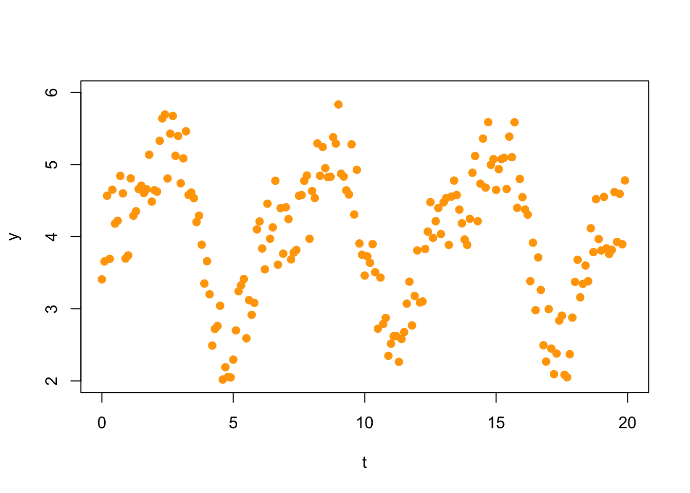
A first Fourier approximation would fit a model of the form \[ f_1(t) = c_0 + c_1 \sin(t) + c_2 \cos(t). \] Thus, we make the following matrix (we show here only the first 10 rows; there are 200 rows).
##       [,1]       [,2]      [,3]
##  [1,]    1 0.00000000 1.0000000
##  [2,]    1 0.09983342 0.9950042
##  [3,]    1 0.19866933 0.9800666
##  [4,]    1 0.29552021 0.9553365
##  [5,]    1 0.38941834 0.9210610
##  [6,]    1 0.47942554 0.8775826
##  [7,]    1 0.56464247 0.8253356
##  [8,]    1 0.64421769 0.7648422
##  [9,]    1 0.71735609 0.6967067
## [10,]    1 0.78332691 0.6216100
Now we solve the normal equations
##            [,1]
## [1,]  3.9971143
## [2,]  1.0207277
## [3,] -0.4486618
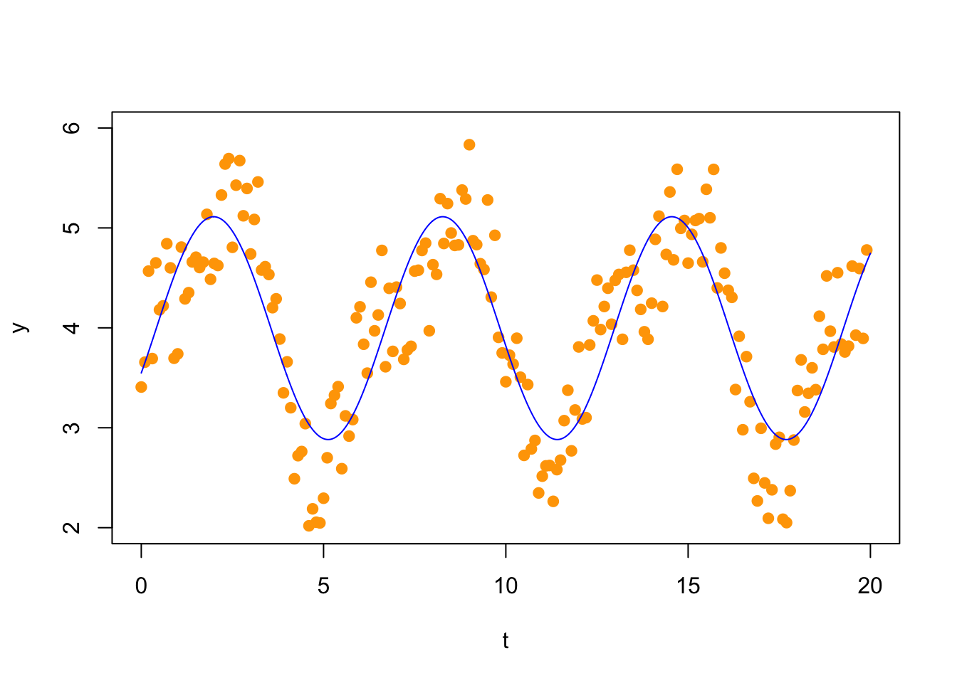
and plot the solution
 Your task:
- Update this to add the second Fourier coefficient terms by fitting the following function to the data. Plot your result. \[ f_2(t) = c_0 + c_1 \sin(t) + c_2 \cos(t) + c_3 \sin(2t) + c_4 \cos(2t) \]
- Compute the length of the residul vector for both the \(f_1(t)\) and the \(f_2(t)\) model. Which approximation looks better visually. That is, does the second approximation capture more of the shape of the data, or do you think that the first is a better model?
8.5 Global Fossil Fuel Emissions
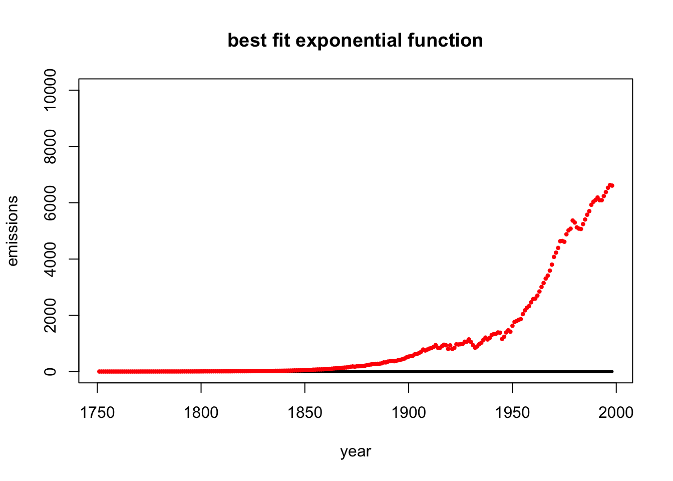
Below is a plot of global fossil fuel emmissions between 1751 and 1998 measured in megatons of carbon.
year=c(1751:1998)
emissions = c(3, 3, 3, 3, 3, 3, 3, 3, 3, 3, 3, 3, 3, 3, 3, 3, 3, 3, 3, 3, 4, 4, 4, 4, 4, 4, 4, 4, 4, 4, 5, 5, 5, 5, 5, 5, 5, 5, 5, 5, 6, 6, 6, 6, 6, 6, 7, 7, 7, 8, 8, 10, 9, 9, 9, 10, 10, 10, 10, 10, 11, 11, 11, 11, 12, 13, 14, 14, 14, 14, 14, 15, 16, 16, 17, 17, 18, 18, 18, 24, 23, 23, 24, 24, 25, 29, 29, 30, 31, 33, 34, 36, 37, 39, 43, 43, 46, 47, 50, 54, 54, 57, 59, 69, 71, 76, 77, 78, 83, 91, 95, 97, 104, 112, 119, 122, 130, 135,
142, 147, 156, 173, 184, 174, 188, 191, 194, 196, 210, 236, 243, 256, 272, 275, 277, 281, 295, 327, 327, 356, 372, 374, 370, 383, 406, 419, 440, 465, 507, 534, 552, 566, 617, 624, 663, 707, 784, 750, 785, 819, 836, 879, 943, 850, 838, 901, 955, 936, 806, 932, 803, 845, 970, 963, 975, 983, 1062, 1065, 1145, 1053, 940, 847, 893, 973, 1027, 1130, 1209, 1142, 1192, 1299, 1334, 1342, 1391, 1383, 1160, 1238, 1392, 1469, 1419, 1630, 1767, 1795, 1841, 1865, 2043, 2177, 2270, 2330, 2463, 2578, 2595, 2701, 2848, 3009, 3146, 3306, 3412, 3588, 3802, 4075, 4227, 4394, 4633, 4641, 4613, 4879, 5018, 5078, 5368, 5297, 5125, 5080, 5067, 5241, 5405, 5573, 5701, 5926, 6035, 6096, 6186, 6089, 6090, 6236, 6378, 6530, 6628, 6608)
plot(year,emissions,pch=20,cex=.7,col="red")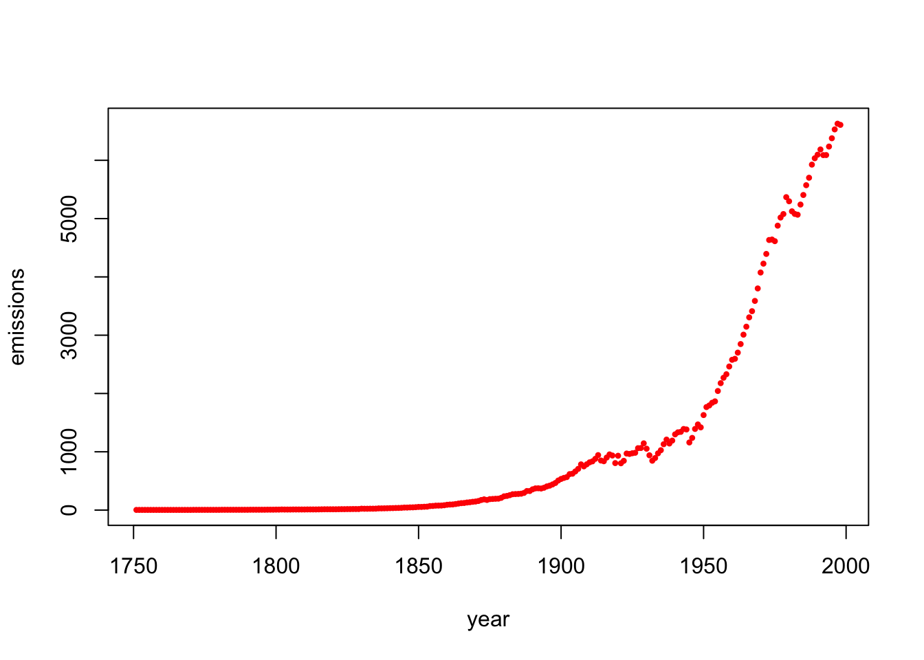
The data suggest that the fossil fuel emissions \(f\) follow an exponential model with respect to the year \(y\): \[f = a e^{k(y-1750)},\] where \(a\) and \(k\) are the unknown constants. This model is not linear in the unknowns \(a\) and \(k\), but (this is a great idea!) it becomes linear if we take the logarithm of both sides. Doing so yields the following linear system: \[\log(f)=\log(a)+k(y-1750).\]
- Note: This process works for any logarithm, but it is common to use the natural logarithm (use
log()in R). - Note: To simplify even further, we will define
time=year-1750so that time represents years after 1750.
This results in the model
\[ \log(f)=d+kt,\] where \(d=\log(a)\) and \(t\) is time (since 1750),
Your task: Use least-squares projection to find the best fitting exponential function for this data. This will give you the values for \(d\) and \(k\), and once you know \(d\), you can find \(a = \exp(d)\). We have started the code for you by defining x=year-1750 and y=log(emissions).
### your code goes here.
# be sure to define d and k and A
t=year-1750
y=log(emissions)
A=cbind(1)  # this isn't right, yet!
d=1
k=0
#####
# your code above has found b and k
(a = exp(d))
## [1] 2.718282## [1] 0Run the code below to plot the original data along with your exponential model curve \(f(t)\). Note: This code assumes that you have already defined the values for k and a. Otherwise, it will not work!
  f=function(y){a * exp(k*(y-1750))}
  plot(year,f(year),type="l",lwd=3,ylim=c(0,10000),ylab="emissions", main="best fit exponential function")
  points(year,emissions,pch=20,cex=.7,col="red")